Table of Content
- History of Regression And Machine Learning
- Regression Analysis To Find Correlation
- Linear Regression in Machine Learning
- Multiple Linear Regression
- Hands-on: python code in Jupyter Notebook
- Advantage, Disadvantage, And Conclusion
Brief history of regression: Sir Francis Galton published a paper called "Regression towards mediocrity in hereditary stature" in 1886 (source: https://en.wikipedia.org/wiki/Regression_toward_the_mean), although he is best known for his development of correlation, most of his work on inheritance led to the development of regression, from which correlation was a somewhat ingenious deduction.
Meanwhile, Arthur Lee Samuel, a computer scientist, is credited with coining the term "Machine Learning" in 1959 (source: https://en.wikipedia.org/wiki/Arthur_Samuel_(computer_scientist)), he created a checker playing program to teach computers to play games.
Regression analysis (source: https://en.wikipedia.org/wiki/Regression_analysis) is a widely used statistical method to ascertain the presence and strength of a relationship between two variables and to understand the what is the relationship.
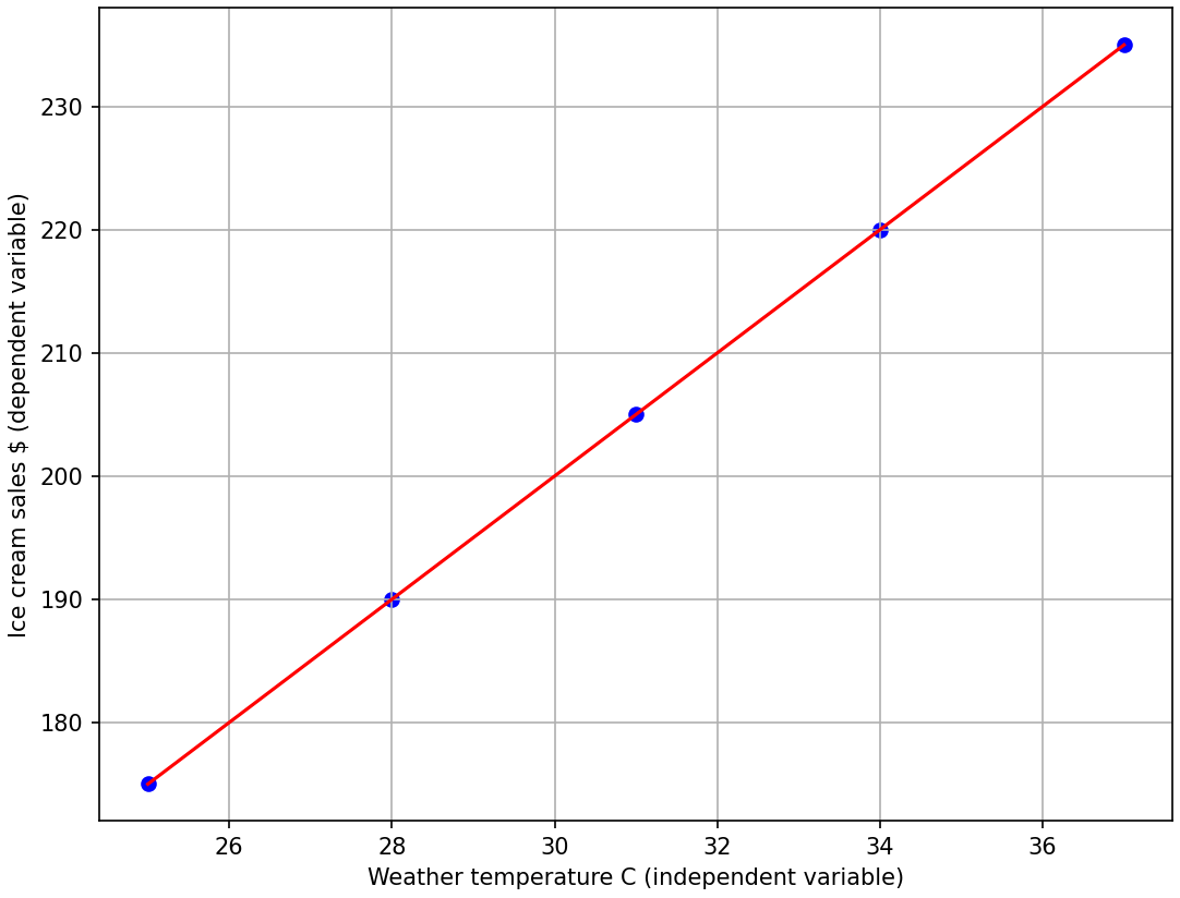
A simple example is to check if there is any relationship between weather temperature and ice cream sales, if we use the data (see the provided code and data) then we can see there is a strong relationship between those values. According to the scatter graph of those values we can see that changes in weather temperature influence ice cream sales, as weather temperatures rise, ice cream sales tend to increase as well. This demonstrates a positive correlation between weather temperature and ice cream sales.
Linear regression is the simplest and fundamental requirement to understand to learn about Machine Learning. As one of the foundational techniques in statistical modeling, linear regression serves as a cornerstone for grasping more complex algorithms in the field of machine learning. Its straightforward approach to modeling the relationship between one or more independent variables (X) and a single dependent variable (y).
The fundamental assumption of linear regression is that this relationship is linear, implying that changes in the independent variable(s) result in proportional changes in the dependent variable. Leveraging this assumption, linear regression constructs a linear equation that best fits the data, enabling predictive analysis and inference within a linear framework. Its applicability spans various industries, making it a vital tool for predictive analytics and data-driven decision-making.
A single independent Linear Regression equation is:
y = (X * coefficient) + intercept
- Intercept represents the predicted value of the dependent variable when the independent variable is zero.
- Coefficient represents the change in the dependent variable for a one-unit change in the independent variable, holding all other variables constant.
We will know the value of Intercept and Coefficient after we built our model using Linear Regression.
Simple numbers (input data) for quick calculation using ice cream sales example:
Weather_temperature = [[25],[28],[31],[34],[37]]
Ice_cream_sales = [[175],[190],[205],[220],[235]]
After we built the model using Linear Regression then we can get these values:
Intercept: 50
Coefficient: 5
Then we can continuously calculate other values such as:
temperature_to_predict = [[38],[39],[40]]
The result:
sales_prediction = [
  [(38 * 5) + 50 = 240],
  [(39 * 5) + 50 = 245],
  [(40 * 5) + 50 = 250]
  ]
Knowing the coefficients and intercept values will enable us to consistently predict new values, ensuring a continuous calculation in the future using linear regression analysis.
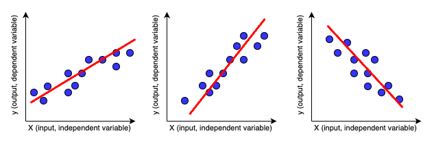
The simple numbers above are used only to understand the formula, the calculation is 100% accurate with 0 (zero) random error, the red line fitting all data points. Prediction using Linear Regression using real-world data may produce some random errors ("noise"), these are samples of visualized data points, the straight red line (the closest Intercept and Coefficient values) is not fitting all the data points, hence we use the word "prediction".
Multiple Linear Regression serves as an extension to simple Linear Regression, addressing the reality of real-world scenarios where multiple independent variables often influence the dependent variable. This makes multiple linear regression an essential tool for predictive analytics and data-driven decision-making across various industries, some examples:
- Predict house prices based on location, total bedrooms, size, proximity to schools, transportation, shopping centers, etc.
- Predict personal insurance cost based on age, gender, occupation, income level, education, main living location (urban, suburban, rural), pre-existing condition, family medical history, etc.
- Predict used-car price based on brand and model, age, mileage, body type, vehicle history, etc.
- Predict sales revenue based on advertising expenditure, pricing strategies, seasons, competitors activities, etc.
- Predict company stock price based on profit margin, financial, company's industry trend, consumer behavior, social media trend, bank interest rate, regulatory environment, geopolitical events, etc.
Multiple independent variables Linear Regression equation is:
y = (X1 * coef1) + (X2 * coef2) + (X3 * coef3) + (Xn * coefn) + intercept
- Intercept represents the predicted value when all the independent variables are zero.
- In multiple linear regression, there is a coefficient for each independent variable.
Hands-on with python code, there are numerous articles on linear regression available online, this brief article aims to provide a hands-on demonstration of implementing linear regression using Python, with the help of scikit-learn, it is simple and easy to use python code to learn Machine Learning for novice software developer. Please find the Python code in Jupyter Notebook, Github: Basic Linear Regression
Advantages of Linear Regression: One of the key advantages of linear regression is its simplicity. The linear relationship between variables is easy to understand and interpret, making it accessible to both beginners and experts alike. Additionally, linear regression provides transparent insights into the relationship between variables, allowing for meaningful interpretation of coefficients and predictions.
Disadvantages of Linear Regression: Despite its simplicity, linear regression has limitations that may impact its performance in certain scenarios. For instance, it assumes a linear relationship between variables, which may not always hold true in real-world data. In cases where the relationship is non-linear, more flexible modeling techniques such as polynomial regression or machine learning algorithms like decision trees or neural networks may yield better results.
In conclusion, the vast landscape of machine learning, mastering linear regression serves as the foundational stepping stone to understanding more complex algorithms. Its simplicity and interpretability provide invaluable insights into the relationships between variables, laying a solid groundwork for delving into advanced techniques.
After we understand the linear regression then the next learning point is how to solve non-linear regression using Polynomial Regression.